Welcome to CINDERellA!

The goal of this project is to enable you to run causal Bayesian networks that accurately predict up and downstream genes and entire regulatory networks on the basis of gene expression or gene expression+genetics.

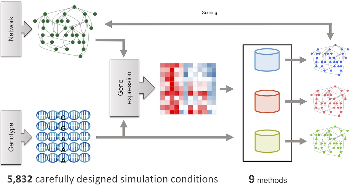
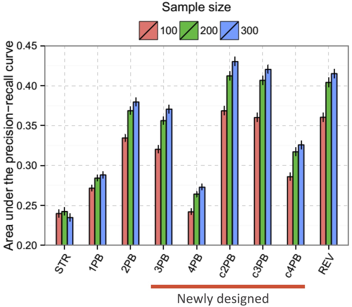
You can read more about methods included in this toolbox in this paper in Genetics where we compare their performance across ~14,000 realistic networks.

CINDERellA has been used to discover genes driving Alzheimer’s disease-related dementias (AD/ADRD) on the basis of bulk brain transcriptomes, brain multi-omics data 1, and brain multi-omics data 2.

Overview

CINDERellA is an easy-to-use Bayesian Network Learning Tool that learns causal networks from gene expression data using Markov Chain Monte Carlo (MCMC) methods.

⚠️ MATLAB Compatibility: This toolbox is compatible with MATLAB versions up to R2016a. Newer MATLAB versions may encounter compatibility issues.

Quick Start

Step 1: Setup

% Add CINDERellA to your MATLAB path
CINDERellA_PATH = './functions';
addpath(CINDERellA_PATH);

Step 2: Load Your Data

% Load expression data (user's responsibility - done outside the function)
expdata = read_exp('your_expression_data.txt');

Step 3: Run CINDERellA

% Basic usage with default parameters
CINDERellA(expdata.data);

Usage Examples

Basic Usage

% Load data first
expdata = read_exp('my_expression_data.txt');

% Run with default settings
CINDERellA(expdata.data);

Custom Parameters

% With custom parameters
CINDERellA(expdata.data, 'output_dir', 'my_results', ...
                'max_parents', 3, 'runtime_minutes', 30, 'num_samples', 1000);

Using Prior Knowledge

% Create prior matrix to constrain search space
nGenes = size(expdata.data, 1);
prior = ones(nGenes, nGenes);  % Start with all edges allowed
prior(1,2) = 0;  % Disallow edge from gene 1 to gene 2
CINDERellA(expdata.data, 'prior_matrix', prior);

Visualization Options

% With layout and visualization options
CINDERellA(expdata.data, 'layout', 'force', 'edge_threshold', 0.33);

Input Parameters

Required

data_matrix - Expression data matrix (rows=genes, columns=samples)

Optional Parameters

‘output_dir’ - Output directory (default: './CINDERellA_results/')
‘sampler’ - MCMC sampler method (default: 'M.c2PB', or 'M.REV50' if prior used)
‘max_parents’ - Maximum parents per gene (default: 3)
‘runtime_minutes’ - Total runtime in minutes (default: 0.5)
‘num_samples’ - Number of network samples to collect (default: 100)
‘edge_threshold’ - Edge frequency threshold for visualization (default: 0.3)
‘prior_matrix’ - nGenes × nGenes binary matrix (1=allowed, 0=disallowed edges)
‘force_recompute’ - Force recomputation even if results exist (default: false)
‘layout’ - Network layout algorithm (default: 'force')

MCMC Samplers

Single Chain Samplers

'STR', 'c2PB', 'c3PB', 'c4PB', '1PB', '2PB', '3PB', '4PB', 'REV50'
Samples networks every (runtime/num_samples) seconds

Multi-Chain Samplers (Recommended)

'M.STR', 'M.c2PB', 'M.c3PB', 'M.c4PB', 'M.1PB', 'M.2PB', 'M.3PB', 'M.4PB', 'M.REV50'
Collects final network state from each chain after (runtime/num_samples) seconds

Layout Options

‘circle’ - Circular layout
‘force’ - Force-directed layout (default)
‘layered’ - Hierarchical layered layout
‘subspace’ - Subspace layout

Data Format Requirements

Input file: Tab-separated text file
Structure: Genes as rows, samples as columns
Minimum: At least 2 genes and 2 samples

Output Files

CINDERellA generates several output files in the specified output directory:

edgefrq.txt - Edge frequencies from sampled networks (main result for evaluation)
Mcmc.mat - All sampled networks
Param.mat - Parameters used in the analysis
LS.mat - Local scores
mcmc_diagnostics.png - Log likelihood trace plot
network_visualization.png - Network plot with edges above threshold

Complete Workflow Example

% 1. Setup
CINDERellA_PATH = './functions';
addpath(CINDERellA_PATH);

% 2. Load data (user's responsibility)
expdata = read_exp('test_data/exp.txt');

% 3. Run CINDERellA
CINDERellA(expdata.data, 'runtime_minutes', 1, 'max_parents', 3);

% 4. Evaluation (done separately)
% Load true network if available
network = read_network('test_data/network.txt', size(expdata.data, 1));

% Load learned edge frequencies
edgefrq_data = dlmread('./CINDERellA_results/edgefrq.txt');
nGenes = size(expdata.data, 1);
edgefrq = sparse(edgefrq_data(:,1), edgefrq_data(:,2), edgefrq_data(:,3), nGenes, nGenes);

% Perform evaluation
[AUCPR, AUCROC] = evaluation(edgefrq, network.data, 'plot', 1);

Tips for Best Results

Runtime Settings

Short test runs: 0.5-2 minutes for initial testing
Production runs: 30-60 minutes for reliable results
Complex networks: Consider longer runtimes for better convergence

Sampling Strategy

Multi-chain samplers (M.* prefix) are generally recommended for final results
Single chain samplers are useful for initial testing to see how much runtime is needed for convergence

Prior Knowledge

Use prior_matrix to incorporate known biological constraints
Set prior(i,j) = 0 to disallow edge from gene i to gene j
Set prior(i,j) = 1 to allow edge (default)

Visualization

Adjust edge_threshold to control network complexity in plots
Higher thresholds show only strongest connections
Lower thresholds show more potential connections

Troubleshooting

Common Issues

Empty data matrix: Ensure your data file loaded correctly
Dimension errors: Check that genes are rows, samples are columns
Prior matrix size: Must be nGenes × nGenes
Memory issues: Reduce num_samples or runtime_minutes for large datasets

Performance Optimization

Start with short runtime for testing
Use appropriate number of samples (100-1000 typical)
Consider your system’s computational capacity when setting parameters

Citation

If you use CINDERellA in your research, please cite:

Tasaki, S., Sauerwine, B., Hoff, B., Toyoshiba, H., Gaiteri, C., & Chaibub Neto, E. (2015). Bayesian network reconstruction using systems genetics data: comparison of MCMC methods. Genetics, 199(4), 973-989. doi:10.1534/genetics.114.172619

Author: Shinya Tasaki, Ph.D. (stasaki@gmail.com)
License: 3-clause BSD License